SOPALE
Sopale Nested
Processing SOPALE Output
Printing
MOZART
TMM (Thermo-mechanical Model)
old SOPALE documentation
Geodynamics home page
sopale_nested input
Originally these parameters were all surface-related. New sections have been added for processes which aren't surface processes.
The parameters for each process are defined within a "section". The start of a section is marked with a keyword. Within a section, input parameters must be in a particular order, but sections may be in any order within the file.
Section keywords:
- ADIABATIC
- ARC
- ARC_DELV
- COMPACTION
- EROSION
- EROSION_OUTPUT
- ISOSTASY
- MATCHANGE
- MATCHANGE_DELV
- PROGRADE
- PTT_TRACK
- MAXPTOUTPUT
- SEDIMENT
- WATERLOAD
- surface strings
- surface strings_v2
- OUTPUTS
ADIABATIC section
This section defines parameters for adiabatic heating.
ADIABATIC
adiabatic_heat
ARC section
The ARC module simulates a volcanic arc using multiple, stacked, arc regions.
ARC
Indicates begin of ARC section
An arc region of the model is defined by lagrangian particles whose mechanical property number is ‘color1’. This is mat1, the original material in the arc region. More than one arc region may be defined, each with its own properties.
Arc regions are specified by material and thermal ‘boxes’ defined in the normal manner in the section of input where these boxes are defined. These boxes will be considered normal Sopale material and thermal boxes unless they contain arc lagrangian particles with mechanical material property ‘color1’ (mat 1). Within the boxes only eulerian elements that contain ‘color1’ lagrangian particles are treated as arc eulerian elements. In cases where eulerian elements contain a mixture of arc (color1) and non-arc lagrangian particles a fraction of the element is calculated based on the fraction of arc lagrangian particles, and arc processes are applied to this fraction of the eulerian element and the arc lagrangian particles. Other materials are unaffected by arc processes
Arc regions evolve by the progressive addition of material whose mechanical property number is ‘color2’. This is mat2 and usually takes the form of an infiltrating melt (e.g. basaltic melt) to the arc region or a metsomatic fluid to other regions.
mat2 is added using a fractional rate of change function (time vs dvdt). That is, dvdt is the fractional volume of mat2 added (delta_volume per unit volume of the arc region/per unit time) (units 1/s). The rate of mass additions is dvdt x mat2_density. The dvdt(t) time function for each arc region is defined in the input.
As mat2 is added the density and volume of mat1 evolve. mat1 therefore becomes a ‘composite material’ reflecting the addition of mat2 to mat1
Conservation of heat
mat2 is added at a high temperature and is assumed to cool to the ambient temperature of the arc region during the timestep. During cooling it releases heat, both specific and latent heat (if it solidifies). The heat released is used to heat the arc region comprising the evolving product of the addition of mat2 to mat1. This consumes specific heat and latent heat if mat1 melts.
The temperature of the 4 corner nodes of each eulerian element are increased by ¼ of the elemental temperature increase calculated by the heat balance.
The properties of mat2 and mat1(including the way it evolves as the composite) are taken to be constant. The user must select a consistent set of properties that represent the average temperature dependence of mat2 and a similar set of properties for the evolving mat1 that represent both its average temperature dependence and the average way its properties change as mat2 is added.
Mixing and Reaction Models
The evolution of mat1 (the composite) as mat2 is added can be either that of a Mixing model or a Reaction model.
Mixing model: volume of mat1 increases by the volume of mat2 that is added and the chemical density evolves as the average density of mat1 (the composite) as mat2 is added. Mass is conserved.
Reaction model: mat2 is assumed to react with mat1 to produce the evolving composite. The evolving chemical density of the reaction product (composite) is specified as input as a function of the fractional amount of mat2 that has been added. Mass is conserved. Therefore the volume of the composite evolves in a manner that conserves mass but it is not the sum of the mat1 and mat2 constituent volumes.
The changing chemical density of the lagrangian particles of mat1 (the composite) is stored as the updated chemical density of the material set that contains color1 (mat1). Owing to the changing density, material sets containing arc color1 (mat1) mechanical materials should be defined separately from other material sets and have only one member (color1 number) in the set.
In both models the volume of each eulerian element (cell) is modified each timestep to reflect the evolving volume of the composite. The volume change is enforced using nodal forces to expand or contract the element.
Restarts:
- All material densities are reset using the material densities in the input file.
- The density of any material containing the color1 of an arc region is reset from the value in the arc restart file.
The rate of change of volume is specified by the time and dvdt values. The function is a step function; it keeps its previous value until the current time exceeds one of the t(i) values, and then the value changes to v(i).
There should be dvdt value for time = 0.0
Initial values of dvdt can be calculated:
- choose a percentage volume change, e.g. volchge = 1% = 1e-2
dvdt = volchge / dt
Each arc region is terminated by [end]. The ARC
section also needs a terminating [end]
color1 color2 dens2 temp2
Properties of the two materials. Only used in the thermal calculations. Thermal properties of mat1 (the composite) used in the finite element calculation are specified in the normal input
Cp1 L1 T1l T1i T1s X1h X1l
properties of mat1 (the composite) used to calculate heat absorbed by the composite and the associated increase in temperature.
Cp2 L2 T2l T2i T2s X2h X2l
properties of mat2 (the added material) used to calculate heat added to the system
Specification of addition of mat2 The rate of addition of mat2 is specified by the time and dvdt values. The function is a step function; it keeps its previous value until the current time exceeds one of the t(i) values, and then the value changes to v(i).
There should be dvdt value for time = 0.0
Initial values of dvdt can be calculated:
- choose a percentage volume change, e.g. volchge = 1% = 1.00d-2
- dvdt = volchge / dt
time(1) time(2) time(3) ...
dvdt(1) dvdt(2) dvdt(3) ...
[reaction_model]
Indicates the begin of reaction_model inputs. Optional. If not present, the mixing model will be used.
this is the reaction model In the reaction case the added mat2 reacts with mat1 to produce a composite (mat3) with a specified progressively changing density. The associated change in the volume of the composite is not known (and is not the volume of mat1 plus mat2), Instead, it must be calculated from the mass balance before and after the reaction: Mass balance equation is:
rho3_final x vol3_initial ( 1 + delta_vol3) = rho3_initial x vol3_initial + rho2 x vol2 (eq. 1)
initial and final are the initial and final values at the beginning and end of the timestep rho3_final is the final density of mat3 (the composite) at the end of the timestep from equation above
vol3_initial is the intial volume of mat3 (the composite) at the beginning of the timestep
delta_vol3 is the fractional change in volume of mat3 (the composite) during the timestep, that is the actual volume change divided by vol3_initial
delta_rho3 is the change in the density of the composite from the beginning to end of the timestep and is specified in terms of the volume of mat2 that is added, delta_vol2 (see eq.4 below)
rho2 is the density of mat2
vol2 is the absolute volume of mat 2 added this timestep
delta_rho3 = rho3_final - rho3_initial
Solving for delta_vol3
delta_vol3 = (delta_rho3/ rho3_final) + (rho2/ rho3_final) x (vol2 / vol3_initial) (eq. 2)
where delta_vol3 is the fractional volume change of the composite. This can also be written as
delta_vol3 = (delta_rho3/ rho3_final) + (rho2/ rho3_final) x delta_vol2 (eq. 3)
where delta_vol2 = (vol2 / vol3_initial) the fractional volume of mat 2 added this timestep with respect to vol3_initial. Note eq.3 takes into account that the effect of adding vol2 of mat2 in causing a change delta_vol3 in the reactant (composite) progressively declines as vol3 increases. This is because vol2 becomes a smaller proportion of the composite.
delta_rho3 must be calculated from the input which specifies the total change in rho3 (rho3_increase) that results from adding a total fractional volume of mat2 (f_tot).
Specify how the density of mat1 (the composite) evolves as mat2 is added
f_tot rho3_increase
It is assumed that the density of the composite changes linearly as mat3 is added and reacts
For each timestep the change in composite density (delta_rho3) is given by
delta_rho3 = rho3_increase x f / f_tot; where f = vol2 / vol3_initial (eq. 4)
That is adding vol2 of mat2 initially changes the density in proportion to the initial volume of mat1 (vol1) but this volume evolves as vol3_initial at the beginning of each timestep. Therefore adding vol2 of mat2 each timestep has progressively less effect on the density change during the reaction because this volume of mat2 represents a progressively smaller fraction of vol3, the volume of mat3.
The process of adding mat2 to the arc region is the same for both the Mixing and Reaction Models. That is, the volume of mat2 that is added per timestep is specified. This volume is distributed uniformly within the arc region initially occupied by mat1 and later occupied by mat3 (the composite). Only the consequences of Mixing vs Reaction of mat2 with mat3 are different.
[end]
Indicates end of reaction_model.
[end]
Indicates end of an arc region.
[end]
Indicates end of the ARC section.
Since: sopale_nested version 2013-11-28_1.0
Changed: sopale_nested version 2013-11-28_2.0
Changed: sopale_nested version 2014-01-26_1.0 added
thermal properties
Changed: May 2015. Added reaction model.
ARC_DELV section
The cell volume changes that result from density changes in an arc can be applied either as forces when solving for velocities in the FE mechanical calculation, or added as vertical velocities after the FE mechanical calculation.
ARC_DELV
value
Default: force
Since: June 2015
COMPACTION section
Since sopale_nested version 2009-07-26_14
COMPACTION
n_compact_mat
compaction_method
compaction_rho_fluid
For each material to be compacted.....
compact_matset_num(i)
compact_or_contract(i)
rho_grain(i) surface_porosity(i) compaction_coeff(i)
EROSION section
This section starts with the word EROSION (on a line by itself).
EROSION
erosion_model
erosion_rate OR erode_p OR dummy
nerode_type nerode_ends
Each nodal position, absolute height h = y(i) along the top surface of the model is potentially subject to erosion (removal of material) or deposition (adding of material). Erosion occurs when y(i) .gt. refh. Deposition occurs when y(i). lt .refh (refh is defined in the file sopale1_plus_i). nerode_type specifies when erosion and deposition will occur.
sopale uses the value of refh to determine whether erosion or deposition is done. If the surface is above refh and erosion is turned on, then the surface will be eroded. Similarly, if the surface is below refh and deposition is turned on, then material will be deposited.
- This is the recommended value when deformation in the model will not propagate to the boundaries.
- removed version 2013-06-28_1.0. Use '3' or '5'.
- This gives no-slope boundaries at the edges for surface processes.
- removed version 2013-06-28_1.0. Use '4' or '6'.
- In LS, no erosion of surface endpoints.
- In any nest, the endpoints are set to values (same position) from LS.
- In LS, erode points 1 and nx by same amount as points 2 and nx1-1, respectively.
- In any nest, the endpoints are set to values (same position) from LS.
- In LS, no erosion of surface endpoints.
- In any nest, an extra value (interpolated from the LS surface) on each side is used, and the concept of an 'endpoint' is gone.
- Since version 2013-09-17_1.0
- In LS, erode points 1 and nx by same amount as points 2 and nx1-1, respectively.
- In any nest, an extra value (interpolated from the LS surface) on each side is used, and the concept of an 'endpoint' is gone.
- Since version 2013-09-17_1.0
er_stablax method_slope_avg
only for erosion_model = 2, 4
In erosion models 2 and 4, slope dependent erosion may lead to node by node (n.b.n) oscillations in the surface (development of a saw tooth surface) which may further lead to 'failure and slumping' of the positive saw teeth.
To reduce the tendency for saw teeth to grow (ie an instability to develop) a small component of numerical diffusion is added to the surface processes in erosion models 2 and 4. The theory behind this Lax stabilization is in W. H. Press et al., Numerical Recipes, p.623-629 (Edition 1) and is implemented in the erosion models using equation 17.1.18. The stabilization allows the erosion to satisfy the Courant condition for stability of the surface.
er_stablax is the diffusion coefficient which determines the amount of diffusion and therefore the numerical smoothing of the surface.
The diffusion of the surface used to stabilize slope-dependent erosion is calculated by the explicit forward differencing finite difference method.
y(i,n+1) - y(i,n) = (dt/dx2) * y(i+1,n) - 2y(i,n) + y(i-1,n)
Where y(i) are the vertical positions of the surface nodes...either the nodes of the FE grid (traditional method) or the surface string (string method) and n is the timestep number.
The left side is the amount of diffusive erosion at node y(i) between timestep n and n+1.
dt is the timestep length (secs)
dx is the horizontal spacing between nodes (metres) (FE grid for traditional and particle spacing on surface string for string method)
The above equation is only convergent/stable for dt/ dx2 < ½
This means that for most choices of dt and dx the above formula has to be multiplied by a factor, er_stablax to ensure stability. This is Lax stabilization. That is
dt/dx2 * er_stablax < ½
or
er_stablax > (dx2) / 2 dt
Example:
dx = 1km = 106m
gives er_stablax ~ 10-5
Note this is the maximum value for stability based on nominal values of dt and dx which the user chooses.
However, in cases where dt varies to satisfy the CFL criterion the maximum value of dt should be used in calculating er_stablax. Smaller values will be stable.
Similarly if dx varies the minimum value of dx should be used to calculate er_stablax.
It is important to remember that numerical diffusive stabilization is only a secondary surface process. The physical erosion is the slope-dependent part. The best choice of er_stablax is that it satisfies the above criterion (the maximum value possible for stability) but that the user value should be as small as possible (factor of 10-2 to 10-3 less if possible) so that diffusion is minimized but the slope-dependent erosion is stabilized and no ``saw teeth`` develop. Essentially, the numerical diffusion is designed to keep the growth of the saw teeth under control
Values if er_stablax that are too large may lead to excessive surface smoothing.
It is IMPORTANT to NOTE that Lax stabilization is only turned on where erosion and deposition are turned on. This means that when using nerode_type 1 or 3 the parts of the surface respectively below refh and above refh will not be subject to Lax stabilization and may develop n.b.n oscillations.
It is therefore recommended to use nerode_type =2, unless users have a special need otherwise.
When users only want surface diffusion and no slope-dependent erosion in erosion models 2 and 4, set erosion_rate = 0 and choose and then TEST a suitably small value of er_stablax. Use nerode_type =2 if diffusion is required everywhere.
In erosion model 4 the climate modulation does not affect the numerical diffusion of the surface. It only modulates the slope-dependent erosion and the sediment deposition.
Erosion Model 4
These inputs are for erosion model 4.
nslope
time_slope_dep_rate(i) slope_dep_rate(i)
nsedfil
time_sedfil_rate(i) sedfil_rate(i)
get_erosion = scalefactor * curr_sedfil_rate * dt_e
where
scalefactor = (dabs(h_e - refh)/1.0d0)
(the 1.0d0 is in units of metres, to make the scale factor dimensionless)
This means that sedimentation rates will be greater in basins where the accommodation space is large and less where there is little accommodation. The sedimentation rate, sedfil_rate, varies according to the time function time_sedfil_rate.
NOTE: 1 cm/yr = 3.17097d-10 m/s
nclimate climate_flag
climate_flag < 10: climate function type 1
In climate function type 1 the spatial variation of the climate function is entirely specified by the user using the inputs listed below.
climate_position(i) climate_value(i)
climate_flag ≥ 10: climate function type 2
Since: April, 2016
Climate function type 2 is an orographic climate function designed for orogen-type models where there is one high elevation orogen. The climate function decreases across the left facing orogenic front to simulate the effect of decreasing orographic precipitation between the orogenic foreland and the elevated platueau which is considered to be in a rain shadow, as is the rest of the model to the right of this location.
The climate function is tuned such that starting at left Eulerian grid boundary the climate_value(1) is 0. It then increases linearly to climate_value(2) (recommended 1.0d0) at a distance delta_climate_position1 to the left of the orogenic front. It then decreases linearly across the orogenic front (region of high elevation) to a position within the orogen at distance delta_climate_position2 to the right of the orogenic front. At this position the climate function has value climate_value(3) (recommended 0.0d0- 0.05d0) and remains at this value to climate-position(4), the right boundary of the Eulerian grid.
In Climate function type 2 Sopale recalculates some input values of the climate function to take into account the evolving model surface configuration, in particular the advection of the position of the orogenic front (x_position_half_surface_max)
Best to use Lagrangian string definition of surface to ensure selection of a single point for x_position_half_surface_max for both LS and SS regions.
climate_position(1) climate_value(1)
climate_position(2) climate_value(2)
climate_position(3) climate_value(3)
climate_position(4) climate_value(4)
delta_climate_position1 delta_climate_position2 ntime_step_climate2
er_max_n
Since: September 6, 2014
The inputs here apply a limit to the calculated erosion value at
each point on the eulerian grid. The limits are applied only when the
top of the eulerian grid is above refh. The calculated
erosion value is usually negative (unless overcome by the er_stablax
term (stab * er_stablax * dt), so the er_max_v(i) values
should be negative in order to be effective. The limiting erosion
rate er_max_v(i) will be multiplied by dt
and then compared to the calculated erosion value.
The dt value used will the value in effect for the
current ALE cycle.
The points below define a time varying maximum erosion rate. The maximum erosion rate used at any time will be interpolated from these values.
er_max_t(i) er_max_v(i)
EROSION_OUTPUT section
EROSION_OUTPUT
Indicates start of section.
X, the surface, and the average erosion will be written to a file
at time steps which are multiples of ts_incr. Averaging
of erosion first starts at time step ts_start;
subsequently it starts after file output. Both X and the
surface values are from the time step at which the file is written.
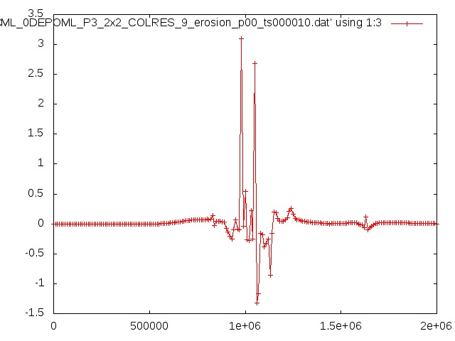
The 'dat' output files can be be plotted using gnuplot; the first
plot command below will generate a plot of the surface. The second
will generate a plot of the erosion. gnuplot can be daunting,
inscrutable, immensely capable, and rewarding. For details, see
/usr/share/doc/gnuplot-doc/html/index.html
dguptill@scram:-sopale_nested$ gnuplot
gnuplot> plot './A19_10DEPCML_erosion_p00_ts000010.dat' using 1:2 with linespoints
gnuplot> plot './A19_10DEPCML_erosion_p00_ts000010.dat' using 1:3 with linespoints
Since sopale_nested version 2011-12-01_7.0
ts_start ts_incr ts_end file_type
The output file name is <nameout1>erosion_p<nn>_ts<tttttt>.<file_type>, where:
tttttt is the time step
ISOSTASY section
This section defines parameters for isostasy. The implementation of flexural isostasy in SOPALE is based on the "beam code" in microfem (an older model code). Explanation of beam, from Juliet Hamilton's notes on microfem.
isost, n_beam_elem, load_extended_beam

  isost
   = 1  use Airy (local) isostasy
   = 11 use Airy (local) isostasy with tangential boundary conditions
   = 2  use flexural isostasy
   = 21 use flexural isostasy with tangential boundary conditions

  n_beam_elem  (only needed for versions code-apr11-05-extbeam and later)
     = the number of elements in the beam (for flexural isostasy)
       This allows the user to make the beam extend beyond the Eulerian
       grid on the right-hand side.  For example, if your Eulerian grid
       is 100 elements wide, then setting n_beam_elem to 200 makes the
       beam twice as wide as your Eulerian grid.  The extra beam length
       extends to the right of your Eulerian grid.

       NOTE: if you are using an extended beam and erosion, it is
       recommended that you set nerode_ends to 0. (nerode_ends is found
       in the EROSION section of surfaceproc_i.)
       You should also check to make sure that your definition of
       the flexural rigidity (see below) covers the entire length of the
       extended beam.

  load_extended_beam (only needed for versions code-apr13-05-extbeamtest and later)
     = 1  Load the extended part of the beam with the same loads as on
          beam element nx-1 (i.e. the rightmost element in the Eulerian grid).
     = 0  Set the load on the extended part of the beam to 0 (zero).

     NOTE: The extended beam is always loaded for the initial isostatic
     adjustment.  For any isostatic calculations during the model run, the
     extended beam is loaded according to the value of load_extended_beam.


rho_below
   Density of the material below the model (i.e. density of material in
   which the model "floats")

If isost=2 or isost=21 (indicating flexural isostasy) then you need the
following additional lines:

nbreak
   Column number for node which defines a break in the beam.
   Beam 1 is the right-hand beam extending from columns nbreak+1 to nx1.
   Beam 2 is the left-hand beam extending from columns 1 to nbreak.
   If you just want one beam, you can use nbreak = 0; this will make
   the entire beam Beam 1.

ibbc(1,k), k=1,4
   Type of boundary conditions for Beam 1 (to the right of nbreak,
   excluding nbreak).
      ibbc(i,1) = deflection or force for left end of beam i
                  0 = imposed deflection  (Dirichlet)
                  1 = imposed force       (Neumann)
      ibbc(i,2) = rotation or moment/torque, left end of beam i
                  0 = imposed rotation       (Dirichlet)
                  1 = imposed moment/torque  (Neumann)
      ibbc(i,3) = deflection or force for right end of beam i
                  0 = imposed deflection   (Dirichlet)
                  1 = imposed force        (Neumann)
      ibbc(i,4) = rotation or moment/torque right end of beam i
                  0 = imposed rotation       (Dirichlet)
                  1 = imposed moment/torque  (Neumann)

bbc(1,k), k=1,4
   Boundary conditions corresponding to the BC flags in the line above,
   e.g. if ibbc(1,1)=1, corresponding to an imposed deflection, then
   bbc(1,1) would be the value of the imposed deflection.

ibbc(2,k), k=1,4
   Boundary conditions for Beam 2 (to the left of nbreak, including nbreak).
   These are defined the same way as for Beam 1 (see above).
   Beam 2 has an additional possible value for ibbc(2,3) corresponding
   to the right-hand end of Beam 2.

   ibbc(2,3) = -1 means that Beam 2 is slaved to Beam 1; the deflection
                  for this end of Beam 2 must have the same deflection
                  as the left-hand end of Beam 1.
                  Note that this imposed value will result in an incorrect
                  overall isostatic balance of loads on Beam 2 in the
                  region of nbreak because the slaved deflection
                  overrides the isostatic balance of Beam 2.

bbc(2,k),k=1,4
   Boundary conditions corresponding to the BC flags in the line above.
   These are defined in the same way as for Beam 1.

nflex
    Number of intervals in the piecewise linear definition of
    the lateral variation of the flexural rigidity of the beams.
    These intervals are defined along the beam, left to right.

For k= 1, nflex, we have:

xflxl(k),xflxr(k),tmpflx(k)
    xflxl(k)  = x coordinate of left end of interval
    xflxr(k) =  x coordinate of right end of interval
    tmpflx(k) = value of flexural rigidity within the interval

    Sopale will use linear interpolation to fill in the flexural
    rigidity values for any sections of the beam which are not covered
    by the intervals defined above.
    Note that the flexural rigidity is constant within any of the
    above defined intervals.  You will need nflex .ge. 2 if you want
    linear interpolation of the flexural rigidity, i.e. not a constant
    value of the whole interval.

ncfb
    Number of lines defining additional loads
    These loads are in addition to the weight of the model, which is
    calculated and applied as equivalent nodal loads on the finite
    element beam. The additional nodal loads represent additional forces
    other than isostatic (buoyancy) forces.

For i=1,ncfb, we have:

node,cfb(2*node-1),cfb(2*node)
     node = column number where the additional beam load is placed
     cfb(2*node-1)  = vertical (z) component of additional load at this node
     cfb(2*node)    = additional torque load at this node


Example:

ISOSTASY
21      ! isost (1=Airy,11=Airy with tangential bcs, 2=flexural, 21=flexural with tangential bcs)
3.3d3    ! rho_below
0        ! nbreak
1 1 1 1         ! (ibbc(1,k),k=1,4)
0.d0 0.d0 0.d0 0.d0    ! (bbc(1,k),k=1,4)
0 0 1 1     ! (ibbc(2,k),k=1,4)
0.d0 0.d0 0.d0 0.d0    ! (bbc(2,k),k=1,4)
1   ! nflex
0.d0  500.d3  1.d22   ! xflxl(k),xflxr(k),tmpflx(k)
1    ! ncfb
1 0.d0 0.d0   ! node,cfb(2*node-1),cfb(2*node)
MATCHANGE section
This section defines parameters for material phase changes.
The traditional (prior to version 2009-07-26_28.0) matchange code uses cell (Eulerian elemental pressures and temperatures interpolated from the nodal values) pressure and temperature when applying matchange rules to a Lagrangian particle.
When sopale_nested is running in nested mode, cell sizes are usually quite different (LS vs SS); hence the cell pressures and temperatures are different. Hence the result of any matchange rule can be different when cell pressures and temperature are used.
Aside from the undesirable model results, this breaks the restart code. For details, see the (closed) ticket describing different temperatures on a restart.
In version 2009-07-26_28.0 (and later), when applying a matchange rule to a Lagrangian particle, there is the option of using a pressure and temperature that are calculated for that particle. When this option is used, the result of the rule should be the same, no matter whether the rule is applied in LS or SS.
Each Lagrangian particle already has a temperature (calculated by
interpolating Eulerian nodal values - t1), so we can use that.
Lagrangian Particle Pressures associated with MATCHANGE
It only remains to select, calculate, and save a pressure for each Lagrangian particle. This is a new array.
When comparing with nature, materials at depth experience the dynamical pressure (mean stress). Therefore the preferred pressure for matchanges that are functions of P,T conditions is mean stress (nodpress contains the Eulerian nodal values)
However, Sopale pressures are sometimes subject to a checkerboard mode which may make nodpress values unreliable and subject to checkerboard errors and flickering between timesteps. Users should use nodpress for the Lagrangian particle pressure unless they experience the checkerboard mode errors. In the latter case it is acceptable to use plitho which is the lithostatic pressures.
MATCHANGE
num_rules_in_file [ PT ]
- dynamical pressures agree to 2 significant digits
- plitho pressures agree to 5 significant digits
- traditional pressures agree to 6 significant digits
For each phase-change rule i, we have the following lines:
color1(i) color2(i) n_vertices(i) set_strain_to_zero(i) [ mech_flag(i) ther_mat1(i) ther_mat2(i) ther_flag(i) ]
If the rule is triggered, any lagrangian particles whose material is mat1(i) will be transformed to material mat2(i). The polygon describes the P-T conditions for triggering the rule.
Since version 2011-12-01_9.3 and 2012-12-21_1.0
The switch matchange_code_version
affects thermal matchanges.
For each vertex j, we have:
phase_change_poly_x(i,j) phase_change_poly_y(i,j)
color_inside_polygon reversible [ ther_mat_inside_polygon ]
The final line of input for each matchange rule
Since version 2012-12-21_1.0
NOTE: The polygon vertices must be specified in counter-clockwise order, and the P-T axes must have the origin at the lower left corner:
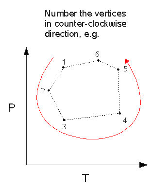
Example:
MATCHANGE
1    ! number of phase-change rules
! 1st mech color, 2nd mech color, # points in polygon, reset_strain
           5               7                5              0
  823.  1.2d9    ! temperature (degrees K), pressure (in Pa)
 1473.  2.5d9    ! temperature (degrees K), pressure (in Pa)
 1473   3.3d10   ! temperature (degrees K), pressure (in Pa)
  623.  3.3d10   ! temperature (degrees K), pressure (in Pa)
  623   3.3d9    ! temperature (degrees K), pressure (in Pa)
7  1    ! mechanical color inside polygon, 1=reversible,0=non-reversible
In this case, the mech color inside the phase-change polygon is 7.
MATCHANGE_DELV section
The cell volume changes that result from color (material) changes can be applied either as forces when solving for velocities in the mechanical FE calculation, or added as vertical velocities after the mechanical FE calculation.
MATCHANGE_DELV
value
Default: force
Since: June 2015
PROGRADE section
This section starts with the word PROGRADE (on a line by itself).
PROGRADE
progradation_model
progradation model 3
no documentation available
progradation models 4 and 7
numprograde
For each time, we need:
tprograde(i), h0(i), hinf(i), x0(i), prograde_length(i), vprograde(i), haggrade(i), vaggrade(i)
NOTE:
- The meaning of haggrade and vaggrade depends on the progradation model. Models 4 and 7 use these number differently. See below.
- All heights and positions are with respect to the origin (x=0, y=0)
- All parameter values are the values for the time interval i and are reset at the beginning of time interval i+1.
- The form of the profile function is quite flexible but it is necessary to the user to calculate the initial values for each time interval carefully if steps/jumps in the positions of the profile are to be avoided. For example, x0(i+1) = x0(i) + vprograde * (t(i+1)-t(i)) correctly positions the profile at the beginning of interval(i+1) to the position it had at the end of interval(i). Similarly, setting haggrade(i+1) to haggradet at the end of the i'th tme interval ensures continuity in the position of haggradet.
- Parameter values specified for tprograde(numprograde) apply for all times larger than this value.
Notes On Progradation Model 4
This is a half-Gaussian progradation, plus uniform aggradation, that vary with time according to a time- stepping function. In progradation model 4 haggrade and haggradet are increments in metres that are added/subtracted from the half gaussian profile at all positions. The general form of the sediment profile function is
  h(x) = (h0(i)-hinf(i)) * exp(-((x-x0(i))**2)/prograde_length(i)**2))
          + hinf(i) + haggrade(i)
The values of h0(i), hinf(i), x0(i), prograde_length(i), and haggrade(i) are reset at the beginning of each time interval(i) and do not vary during the time interval.
During the time interval x0(t) and haggrade(t) vary with time since the beginning of the time interval according to
  x0(i, deltat) = x0(t=t(i)) + vprograde(i) * deltat
  haggrade(i,deltat) = haggrade(t=t(i)) + vaggrade(i)*deltat

  where
    deltat is the time elapsed since the beginning of this time interval
    t(i)   is the absolute model time at the beginning of the time interval
Notes On Progradation Model 7
This is a half-Gaussian progradation, plus local aggradation, that vary with time according to a time- stepping function. In progradation Model 7 haggrade and haggradet are absolute values in metres of the progradation/aggradation profile such that the profile is set to haggradet whereever it is less than haggradet.
haggrade is the initial height of haggradet for each time interval and haggradet is raised or lowered at vaggrade with time. This means the effect of aggradation only occurs where haggradet is greater than the progradation profile.
For example, the seaward end of the progradation profile can be independently determined by aggradation if hinf is set to a value that is less than haggrade. Variations in haggradet will then specify the profile at the seaward end and not hinf provided haggradet remains greater than hinf.
The general form of the sediment profile function is
   h(x) = (h0(i)-hinf(i)) * exp(-((x-x0(i))**2)/prograde_length(i)**2))
          + hinf(i)

   if h(x) is greater than haggradet.
      h(x) is set to haggradet where h(x) is less than haggradet.
The values of h0(i), hinf(i), x0(i), prograde_length(i), and haggrade(i) are reset at the beginning of each time interval(i) and do not vary during the time interval. During the time interval x0(t) and haggrade(t) vary with time since the beginning of the time interval according to
  x0(i, deltat) = x0(t=t(i)) + vprograde(i) * deltat
  haggrade(i,deltat) = haggrade(t=t(i)) + vaggrade(i)*deltat

  where
    deltat is the time elapsed since the beginning of this time interval
    t(i) is the absolute model time at the beginning of the time interval
progradation model 5
no documentation available
progradation model 9
no documentation available
progradation model 10, 11, 12, 13
notes (pdf)
progradation model 14
numprograde
For each prograde interval:
tprograde(i), vprograde(i), haggrade(i), vaggrade(i)
x(1) x(2) ...
level(1) level(2) ...
PTT_TRACK section
This section defines the Lagrangian particles to be tracked during the model run. When a Lagrangian particle is "tracked", its pressure and temperature are periodically saved to a file, for use in PTt (Pressure-Temperature-time) plots.
PTT_TRACK
Indicates start of section.ptt_track_flag
num_tracked_ptcls save_ptt_interval dens_ptt
For i = 1 to num_tracked_ptcls, there should be a line specifying each Lagrangian particle to be tracked:
ptcl_col(i) ptcl_row(i)
When tracking is on, Sopale will create files called ptt_p_c#_r# (where c#_r# is the row number, column number), one file for each tracked particle. Within the ptt_p_c#_r# file, each line has the following values:
| Column | Value |
|---|---|
| 1 | timestep |
| 2 | time in millions of years |
| 3 | temperature in Celsius |
| 4 | dynamic pressure (epress*) divided by 10**8, => it is in kbars |
| 5 | x position of particle (in km) |
| 6 | y position of particles (in km) |
| 7 | depth of particle (in km) |
| 8 | "static pressure" (in kbar), calculated from dens_ptt, assuming the overburden is uniformly of this density. |
| (this is a very approximate pressure estimate). | |
| 9 | dynamic pressure (epress*) at the centre of the Eulerian element where this particle is found (in Pa) |
| 10 | lithostatic pressure (plitho*) at the centre of the Eulerian element where this particle is found (in Pa) |
| 11 | thermal material |
| 12 | density of the thermal material |
| 13** | maximum temperature (Celcius) |
| 14** | maximum dynamic pressure |
| 15** | maximum static pressure |
* epress and plitho are the names of the variables within Sopale; epress corresponds to dynamic pressure; plitho corresponds to lithostatic pressure. They will be good estimates of the dynamic pressure and weight of the overburden (including topography) experienced by the Lagrangian particle if the vertical spacing of the Eulerian grid is small.
** Since version 2009-07-26_22.7
MAXPTOUTPUT section
MAXPTOUTPUT
Records maximum pressure and temperature events for lagrangian particles.
ts_start ts_mod ts_end
ts_mod. The updating will start at
ts_start and terminate at ts_end.(output interval specifications)
There are two ways of specifying when the output files will be written
ts1 ts2 ts3 ...
SameAsNsave2
xul yul xbl ybl
xbr ybr xur yur
screen_factor
screen_factor can be used to avoid that
contamination.
If (dynamical_pressure > screen_factor x
lithostatic_pressure) thenAll lagrangian particles inside the box defined by the 4 points will be tracked. As particles enter the box, they will be added to the tracked list. As particles leave the box, they will be removed from the tracked list.
For each lagrangian particle within the box defined by the user, these data items will be recorded:
| Data Item | Accompanying Data |
|---|---|
| number of the lagrangian particle | |
| model time of output file | |
| x, y coordinates at 'model time' | |
| maximum lithostatic pressure | time, temperature |
| maximum dynamical pressure | time, temperature |
| maximum temperature | time, lithostatic pressure, dynamical pressure |
For example:
#  lag number   model time    lag x pos    lag y pos   plitho_max         time  temperature   pdynam_max
       843590   0.1250E-01   0.9000E+03   0.6204E+03   0.1095E+01   0.1250E-01   0.5442E+03   0.0000E+00
       843591   0.1250E-01   0.9000E+03   0.6198E+03   0.1117E+01   0.1250E-01   0.5511E+03   0.0000E+00

         time  temperature   temper_max         time       plitho       pdynam
   0.0000E+00   0.0000E+00   0.5442E+03   0.1250E-01   0.1095E+01   0.1435E+01
   0.0000E+00   0.0000E+00   0.5511E+03   0.1250E-01   0.1117E+01   0.1453E+01
| pressure | GPa | (sopale_nested uses Pa) |
| temperature | C | (sopale_nested uses K) |
| time | Myr | (sopale_nested uses s) |
| x | km | (sopale_nested uses m) |
| y | km | (sopale_nested uses m) |
Since version 2011-12-01_8.0
SEDIMENT section
This section starts with the word SEDIMENT (on a line by itself).
SEDIMENT
nsedcolor
For each time/sediment material data line:
tchron_strat(i) sedcolor(i) [ sedcolort(i) ]
Since sopale_nested version 2009-07-26_18,
sedcolort(i) is an optional parameter.
WATERLOAD section
This section starts with the word WATERLOAD.
waterloading  = 1 use nodal weights for water loading
              = 0  don't use water loading

refh_water, rho_water, stab_waterweight
    refh_water  = sea level (for code-sep17-03, assumed to be parallel
		  with the x axis)
    rho_water   = density of water
    stab_waterweight = stabilization factor for the water weight
                       (versions code-dec04-03 and later)

NOTE: code-sep17-03 version has modified water loading to act as
      a pressure normal to the (land) surface.  This only works
      if the model is constructed in the x-z coordinate system
      such that the surface of the water (refh_water) is horizontal
      (i.e. parallel to the x coordinate axis) and that gravity acts
      in the minus z direction.
      [ Will only work if ang_gravity is -90.]
OUTPUTS section
Since sopale_nested version 2011-09-06_1.0
OUTPUTS
x_begin x_end flag frequency
Defines a range in x within which lagrangian densities are printed to a file. The filename will be
<nameout1><process_number>.lag_density
where 'process_number' is 0 for LS, and a positive integer for any nest.
Each line of the file, for each time step, for each lagrangian particle, will contain:
- lag number
- x coordinate
- y coordinate
- depth (below surface)
- mechanical color
- density
[surface_strings]
Since sopale_nested version 2014-04-24_1.0
Discontinued sopale_nested version 2016-01-28
Surface process calculations - erosion, sedimentation, progradation, surface advection - can be performed on the top of the eulerian grid. This is the default.
If this section is present, those calculations will be performed on two strings of lagrangian-like particles.
Two strings are maintained; one for the surface, and one for the sediment base. The surface string is the surface of the eulerian grid. The sediment base string is the initial eulerian grid top, modified during time stepping by eulerian velocities - but not affected by surface processes.
These particle strings are initially formed from a copy of the top of the lagrangian grid. The initial spatial density is then increased by a user-specified factor. During time-stepping, the particles move with a velocity in both x and y interpolated from neighbouring points on the eulerian grid. A minimum spacing of particles is maintained by injecting new particles if required.
[surface_strings]
sep_min sep_max
[end]
[surface_strings_v2]
Since sopale_nested version 2016-01-28
Surface process calculations - erosion, sedimentation, progradation, surface advection - can be performed on the top of the eulerian grid. This is the default.
If this section is present, those calculations will be performed on two strings of lagrangian-like particles.
Two strings are maintained; one for the surface, and one for the sediment base. The surface string is the surface of the eulerian grid. The sediment base string is the initial eulerian grid top, modified during time stepping by eulerian velocities - but not affected by surface processes.
These particle strings are initially formed from a copy of the top of the lagrangian grid. The initial spatial density is then increased by a user-specified factor. During time-stepping, the particles move with a velocity in both x and y interpolated from neighbouring points on the eulerian grid. A minimum spacing of particles is maintained by injecting new particles if required.
[surface_strings_v2]
separation
[end]
This page was last modified on Wednesday, 20-Apr-2016 11:02:42 ADT
Comments to geodynam at dal dot ca