sopale_nested input
sopale_nested input is organized into a number of sections; each
section begins with an identifier or keyword. The sections can be in
any order and there can be blank lines in between each section.
Section keywords:
EGRID
EGRID
Sopale requires this section. It defines the Eulerian
grid. The first line of this section is the word EGRID (on a
line by itself).
xor lhoriz nlayers nbzeremesh
xor
x origin, in meters [MUST BE ZERO]
lhoriz
grid width, in meters
nlayers
number of layers with different spacing in grid
nbzeremesh
row number in Eulerian grid, above which grid is uniformly
dilated (stretched) during Eulerian regridding to account for
changes in the top or bottom surfaces. Generally chosen to
match a change in the vertical refinement of the Eulerian
grid. See subroutine zeremesh. When the whole grid is
vertically dilated nbzeremesh = ny (total number of nodes
vertically in the Eulerian grid.) Must be greater than the
row number of the lowest interface (see row_interface
below).
height(1) height(2) ... height(nlayers+1)
height(i)
height (in meters) of the layer interfaces (i.e. heights of the
boundaries between the layers). These are defined from top to
bottom, where the bottom is at height 0.
elements_in_layer(1) elements_in_layer(2) ... elements_in_layer(nlayers)
elements_in_layer(i)
number of elements in layer i. Note that the layers are
numbered from top to bottom.
refh
refh
reference height for erosion
NOTE: refh is used only for erosion. The other erosion
parameters are defined in surfaceproc_i, in the EROSION section.
n_interface
n_interface
number of interfaces (internal surfaces) which will be
advected, or "tracked". You must specify at least one
interface, which is the surface.
For each interface
interface_row(i) apply_surfproc(i)
interface_row(i)
row number of this interface. Rows are numbered from the top down.
apply_surfproc(i)
flag to indicate whether to apply surface processes
(erosion, progradation, etc.) to this surface
0 => don't apply surface processes
1 => apply surface processes
ETEMP
ETEMP
Indicates start of section.
Here the initial Eulerian thermal structure is defined.
Sopale versions prior to 2009-07-26_29.0 require this section.
Versions 2009-07-26_29.0 (and later) do not use this
if type_bct0=3 and
temperature_initial is greater than 0.0 .
If you are using type_bct0=3
the temperature field defined here may be used as a starting
point.
Note that the ETEMP values for temperature will be overwritten
if type_bct0=3.
The type_bct0=3 temperatures will be overwritten if
EPERTURB-T is present.
For more about temperature initialization,
see here.
nlt
nlt
number of layers in the thermal grid
For each layer
ytop(i) ylthick(i) rada(i) cond(i) temptopK(i) qbase(i)
ytop(i)
position of top interface of layer in model coordinate system
ylthick(i)
thickness of layer
rada(i)
radioactive heat generation, A, ie production per unit volume
cond(i)
thermal conductivity of layer
temptopK(i)
temperature of upper interface of the layer (Kelvin)
qbase(i)
vertical heat flux into the base of the layer
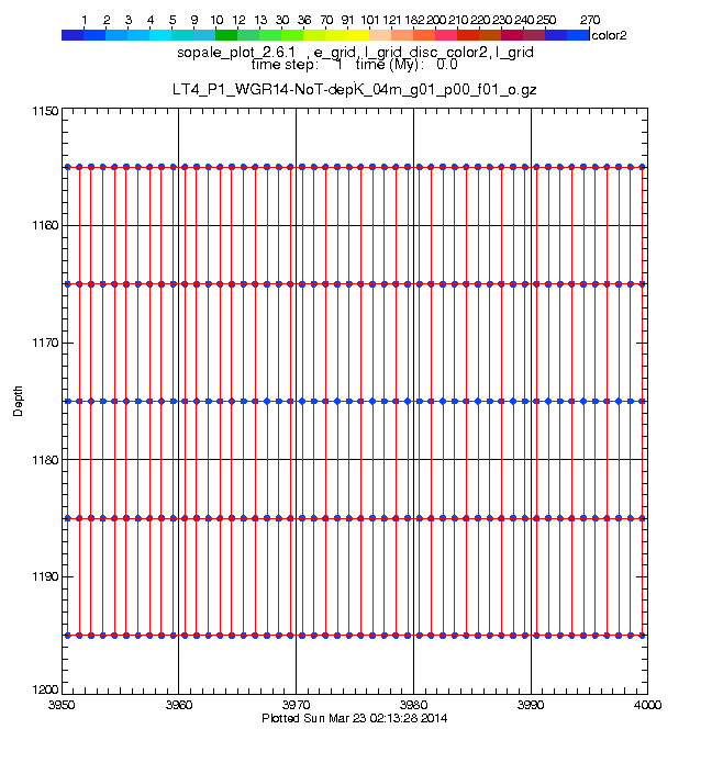
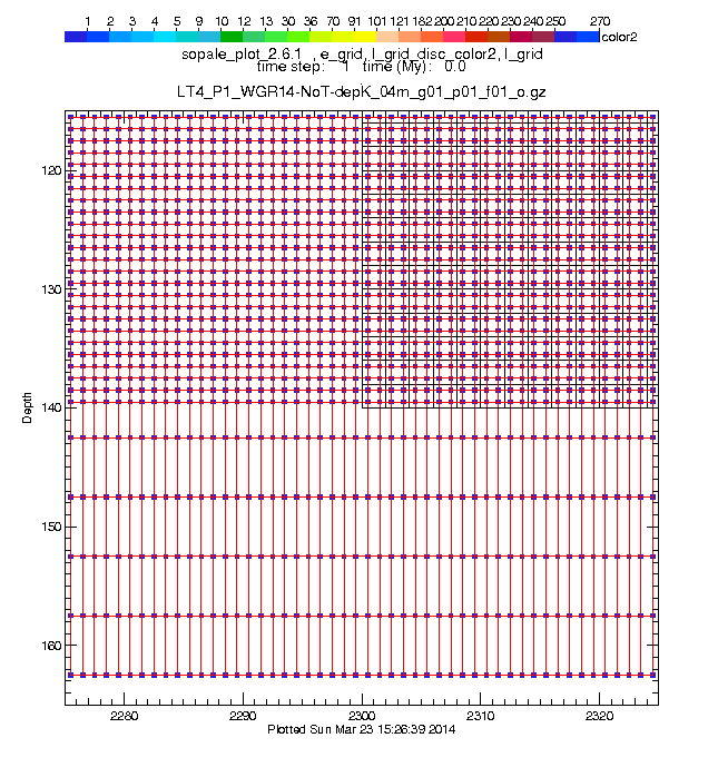
LGRID
LGRID
Indicates start of section.
This section defines the Lagrangian grid. sopale_nested
versions prior to 2014-03-13 require this section. Subsequent
versions accept LGRID_AUTO as an alternative.
xor lhoriz nlayers
xor
x origin, in meters
lhoriz
grid width, in meters
nlayers
number of layers with different spacing in grid
height(1) height(2) ... height(nlayers+1)
height(i)
height (in meters) of the layer interfaces (i.e. heights of the
boundaries between the layers). These are defined from top to
bottom, where the bottom is at height 0.
elements_in_layer(1) elements_in_layer(2) ... elements_in_layer(nlayers)
elements_in_layer(i)
number of elements in layer i. Note that the layers are
numbered from top to bottom.
An example:
LGRID
-1000000. 5000000 3      ! xor    lhoriz  nlayers
1200000 1060000 520000 0 ! yl(i):  height at the top of each layer
140 108 52               ! nyl(i): number of elements in each layer
|
LS upper-left |
LS lower-right |
nest lower-left |
LGRID_AUTO
LGRID_AUTO
Indicates start of section.
sopale_nested will generate a Lagrangian grid, using the
structure (layers) of the eulerian grid. The grid will be (just
barely) all inside the eulerian grid. It will look like injected
lags. Its density will be adjusted for the densest nest.
This is an alternative to the LGRID section.
Since: version 2014-03-13_1.0
left_extension right_extension
left_extension
Length (in m) that will be added to the left edge of the
Eulerian grid when generating the Lagrangian grid.
right_extension
Length (in m) that will be added to the right edge of the
Eulerian grid when generating the Lagrangian grid.
pts_per_cell_x pts_per_cell_y
pts_per_cell_x
number of lagrangian points (in x) generated in each eulerian
cell. This number will be multiplied by the largest nest
magnification in x.
pts_per_cell_y
number of lagrangian points (in y) generated in each eulerian
cell. This number will be multiplied by the largest nest
magnification in y.
An example:
LGRID_AUTO
1000.d3 0.0    ! left and right extension beyond the eulerian grid
2 2            ! number of lags (in x and y) in each eulerian cell
|
LS upper-left |
LS lower-right |
nest lower-left |
LGRID_EXTENSION
Indicates start of section. If extending on both sides of the
lagrangian grid, include one section for each extension.
Since: December 2014
Extending The Lagrangian Grid On A Restart
On a restart, the Lagrangian grid can be redefined and/or
extended. Provided the parts involved are outside the eulerian
grid. Either left or right side.
The extension of the lagrangian grid is created using parameters
from the input file; currently either LGRID
or LGRID_AUTO.
Fast-Forward-In-Time
A transformation, designed to achieve the same result as if the
extension had been included in the original Lagrangian grid
definition, is applied to the extension. After creation:
- the extension is stretched/shrunk vertically by the same
amount that the original grid particles have been moved.
- the extension is stretched/shrunk vertically (preserving
vertical spacing) to match the surface.
- the extension is moved horizontally by the same amount that the
original grid particles have been moved.
After Extension
After the grid has been extended on the left side, the
column and row of individual particles (as used
by pttpaths), will
change.
Limitations (before June 2015)
There is a combination of input parameters for sopale_nested that
will prevent the LGRID_EXTENSION code from working. That
combination is changing
the nest magnification (on
a restart) in a model that
uses LGRID_AUTO.
Why?
LGRID_EXTENSION is another name for 'new model from old'. The
code for it needs the lagrangian grid parameters.
When LGRID_AUTO is used, the lagrangian grid parameters are
deduced from
- the eulerian grid
- the nest magnification.
If the nest magnification is changed (on a restart), the definition
of the lagrangian grid is changed / corrupted, and the
LGRID_EXTENSION code fails.
Parameters
side length
side
'left' => extend the lagrangian grid on the left side.
'right' => extend the lagrangian grid on the right side.
length
the length (meters) of the extension.
x(1) x(2) ... x(n)
x(i)
x(i), i=1,n: x value (meters) of the points (top of grid) to be (re)defined.
In a left extension, x = 0 corresponds to the left edge of the existing lagrangian grid. Negative x values should extend to 'length'. Any positive x values will over write the existing grid.
In a right extension, x = 0 corresponds to the right edge of the existing lagrangian grid. Positive x values should extend to 'length'. Any negative x values will over write the existing grid.
t(1) t(2) ... t(n)
t(i)
t(i), i=1,n: offsets (meters) from the original top of grid.
mechanical boxes
Indicates start of mechanical color boxes. For each box,
include 3 lines. In order to ensure that all the new lags are given a color, the x values of the boxes should cover the range of the top-of-grid values above. The y values should cover the range from 0 (bottom) to the current top of the lagrangian grid plus the maximum of the t(i) above. Note the order of box corners.
- x1 y1 x4 y4
- x2 y2 x3 y3
- color
x1 y1 x4 y4
x1 y1
coordinates of upper left corner
x4 y4
coordinates of upper right corner
x2 y2 x3 y3
x2 y2
coordinates of lower left corner
x3 y3
coordinates of lower right corner
color
color
the mechanical color number assigned to all Lagrangian
particles in this box
[end]
Indicates end of mechanical boxes.
thermal boxes
Indicates start of thermal color boxes. For each box,
include 3 lines. In order to ensure that all the new lags are given a color, the x values of the boxes should cover the range of the top-of-grid values above. The y values should cover the range from 0 (bottom) to the current top of the lagrangian grid plus the maximum of the t(i) above. Note the order of box corners.
- x1 y1 x4 y4
- x2 y2 x3 y3
- color
x1 y1 x4 y4
x1 y1
coordinates of upper left corner
x4 y4
coordinates of upper right corner
x2 y2 x3 y3
x2 y2
coordinates of lower left corner
x3 y3
coordinates of lower right corner
color
color
the thermal color number assigned to all Lagrangian
particles in this box
[end]
Indicates end of thermal boxes.
Coordinate System
When defining the top of an extension and color boxes, the x axis
origin is at the edge of the original lagrangian grid.
For a left side extension, x will range between the
negative of the length of the extension and zero, when only adding to
(not redefining) the grid. When redefining the grid, some x values
will be positive.
For a right side extension, x will range between zero and
the length of the extension, when only adding (not redefining) the
current grid. When redefining, some x values will be negative.
sopale_nested will object, and stop, if the extension includes any
part of the lagrangian grid that has entered the eulerian grid.
The y axis coordinates are same as for the initial lagrangian grid,
modified by the offsets defined for this extension.
Left Side Example
The input below will redefine the leftmost 500 Km, and add another
1000 Km to the left edge of the Lagrangian grid.
For the area between -1000 Km and -500 Km; in the upper 320 Km,
lags are given mechanical color 102 and thermal color 2. In the lower
900 Km, lags are given mechanical color 100 and thermal color 1.
For the area between -500 Km and +500 Km, lags are given mechanical
color 103 and thermal color 3.
LGRID_EXTENSION
! which side is the extension on, and the length of the extension.
        left                             1000.d3
!
! x coordinates of the top of grid (see Coordinate System)
-1000.d3   -750.d3   -500.d3   -250.d3   0.d3   250.d3   500.d3
!
! offsets applied to the y coordinates of the top of grid (a 20 Km bump)
  0.d3       10.d3     20.d3     20.d3   0.d3    0.d3      0.d3
!
! coordinates for the mechanical and thermal boxes:
! For the range of x coordinates, see Coordinate System
! The range of y coordinates is same as the initial Lagrangian grid,
! modified by the offsets above.
!
mechanical boxes
-1000.d3  1220.d3  -500.d3  1220.d3
-1000.d3   900.d3  -500.d3   900.d3
100
-1000.d3   900.d3  -500.d3   900.d3
-1000.d3     0.d3  -500.d3     0.d3
102
-500.d3   1220.d3   500.d3  1220.d3
-500.d3      0.d3   500.d3     0.d3
103
[end]

thermal boxes
-1000.d3  1220.d3  -500.d3  1220.d3
-1000.d3     0.d3  -500.d3     0.d3
1
-1000.d3  1220.d3  -500.d3  1220.d3
-1000.d3   900.d3  -500.d3   900.d3
2
-500.d3   1220.d3   500.d3  1220.d3
-500.d3      0.d3   500.d3     0.d3
3
[end]
Right Side Example
The input below will add 500 Km to the right side of the lagrangian
grid.
LGRID_EXTENSION
! which side is the extension on, and the length of the extension.
        right                             500.d3
!
! x coordinates of the top of grid (see Coordinate System)
0.d3   250.d3   500.d3
!
! offsets applied to the y coordinates of the top of grid (a 20 Km slope)
0.d3    10.d3    20.d3
!
! coordinates for the mechanical and thermal boxes:
! For the range of x coordinates, see Coordinate System
! The range of y coordinates is same as the initial Lagrangian grid,
! modified by the offsets above.
!
mechanical boxes
0.d3  1220.d3      250.d3  1220.d3
0.d3     0.d3      250.d3     0.d3
100
250.d3  1220.d3    500.d3  1220.d3
250.d3     0.d3    500.d3     0.d3
101
0.d3   600.d3      500.d3   600.d3
0.d3     0.d3      500.d3     0.d3
103
[end]

thermal boxes
0.d3  1220.d3      250.d3  1220.d3
0.d3     0.d3      250.d3     0.d3
1
250.d3  1220.d3    500.d3  1220.d3
250.d3     0.d3    500.d3     0.d3
2
0.d3   600.d3      500.d3   600.d3
0.d3     0.d3      500.d3     0.d3
3
[end]
EPERTURB
EPERTURB
This section defines the perturbation of the Eulerian grid,
including any definition of the initial surface. If you don't
want any perturbation for the Eulerian grid, just leave this
section out entirely. (This section and the LPERTURB section
replace the old initsurf_i file.). The first line of this
section is the word EPERTURB (on a line by itself).
nperturb
nperturb
= number of rows to perturb.
For each row to be perturbed, supply (at least) the row number
and type of perturbation.
row_number(i) type_perturb(i)
row_number(i)
= row to perturb. Row numbers start at the top, and
increase downwards.
type_perturb(i)
= type of perturbation to apply.
Additional inputs may be required, depending on type_perturb(i).
type_perturb(i) = 0
No perturbation done. Do not provide any inputs.
type_perturb(i) = 1 Sinusoidal perturbation.
xsleft_surf xsright_surf amp_surf wavl_surf decayl_surf ymid_sin
xsleft_surf
= left endpoint of sinuosoidal surface topography
xsright_surf
= right endpoint of sinuosoidal surface topography
amp_surf
= amplitude of sine wave
wavl_surf
= wavelength of sine wave
decayl_surf
= length scale over which the amplitude of the sine wave
decays to zero adjacent to xsleft_surf and
xsright_surf
ymid_sin
= y position of midline of sine wave. Choose this value so
that ymid_sin + amp_surf is equal to or less than the
height of the Eulerian grid.
type_perturb(i) = 2 Lehner Normal perturbation (for progradation)
h0 hinf x0 prograde_length h0star
h0
= surface height at x=0 (metres)
hinf
= limit of surface height at x = infinity (metres)
x0
= initial x position where surface height is at
(h0-hinf)/2 + hinf (metres)
prograde_length
= width of the distribution (metres) defined by
h(x) =
              (h0-hinf)exp(-((x-x0)**2)/prograde_length**2) + hinf
h0star
= lowered height behind the prograding surface
type_perturb(i) = 3 Level-slope-level perturbation
x1 level1 x2 level2
x1
= x position of start of slope section
level1
= y (or temperature) position of start of slope section
x2
= x position of end of slope section
level2
= y (or temperature) position of end of slope section
For x < x1, y will be set to level1.
For x > x2, y will be set to level2.
A straight-line segment joins (x1,level1) and (x2,level2).
type_perturb(i) = 4 Level-slope-slope-slope-level perturbation
x1 level1 x2 level2 x3 level3 x4 level4
x1
= x position of start of slope section.
level1
= y (or temperature) position of start of slope section
x2
= x position of 1st intermediate point.
level2
= y (or temperature) position of 1st intermediate point
x3
= x position of 2nd intermediate point.
level3
= y (or temperature) position of 2nd intermediate point
x4
= x position of end of slope section.
level4
= y (or temperature) position of end of slope section
For x < x1, y (or temperature) will be set to level1.
For x > x4, y (or temperature) will be set to level4.
Straight lines join (x1,level1) and (x2,level2) and (x3,level3) and (x4,level4).
Implemented version 2009-07-26_9.
type_perturb(i) = 5 <n> point perturbation. A
generalization of type_perturb 3 and 4.
number_of_points
For each perturbation point, supply x and the value at that point.
x(i) level(i)
x(i)
= x at position i.
level(i)
= y (or temperature) at position i.
For x < x(1), y (or temperature) will be set to level(1).
For x > x(n), y (or temperature) will be set to level(n).
Straight lines join (x(1),level(1)) and (x(2),level(2)) and...and (x(n-1),level(n-1).
Implemented version 2009-07-26_22
remeshbottom
remeshbottom
= row number in grid (counting from the top), above which the
vertical grid spacing is dilated or compressed to accomodate the
perturbations specified; at this row and below, the grid spacing
is not affected. NOTE: make sure you choose remeshbottom to be
further down than the lowest point of your defined surface
topography.
Last line of the EPERTURB section.
LPERTURB
LPERTURB
This section defines the perturbation of the Lagrangian grid.
If you don't want any perturbation for the Lagrangian grid,
just leave this section out entirely. (This section and the
EPERTURB section replace the old initsurf_i file.).
The first line of this section is the word LPERTURB (on a
line by itself). This section is optional.
Same variables as EPERTURB
EPERTURB-T
EPERTURB-T
The first line of this section is the word EPERTURB-T (on
a line by itself). This section is optional.
This section perturbs (modifies) the existing Eulerian
temperature field, which could be either the result of ETEMP or
the steady-state calculation. For more on the theory, see here.
Implemented version 2009-07-26_22.4
x1_pert level1 x2-pert level2 isothermk_pert adiabat_opt
x1_pert
x1_pert and x2_pert split the base
of the Eulerian grid into three sections.
level1
perturbation level for x < x1_pert
x2-pert
x1_pert and x2_pert split the base
of the Eulerian grid into three sections.
level2
perturbation level for x > x2_pert
isothermk_pert
The isotherm (Kelvin) to which the perturbation is applied.
adiabat_opt
Set this below, or equal to, 1.0d-12
CRPIT
CRPIT
Defines the CRPIT parameters. CRPIT=Controlled Remeshing with
Partial Interface Tracking. See CRPIT
notes for a more detailed explanation. The CRPIT notes
explain the concept of controlled remeshing and partial
interface tracking, the meaning of the control function and the
definitions of Regions 1, 2, 3, and 4.
The first line of this section is the word CRPIT (on a line by
itself). This section is optional.
crpit_interface stablax_interface
crpit_interface
number of the tracked interface to which you want to apply CRPIT
stablax_interface
lax stabilization parameter to use for the CRPIT interface.
If you don't want to use any lax stabilization, use
stablax_interface = 0.d0
crpit_x1 crpit_x2 crpit_x3
crpit_x1
x value which defines the boundary between Region 1 and Region
2 of the CRPIT control function at time=0.
crpit_x2
x value which defines the boundary between Region 2 and Region
3 of the CRPIT control function at time=0.
crpit_x3
x value which defines the boundary between Region 3 and Region
4 of the CRPIT control function at time=0.
crpit_f_fraction
crpit_f_fraction
the fractional value of the CRPIT control function in Region 1.
crpit_f_velocity
crpit_f_velocity
the velocity at which the CRPIT control function is moving
crpit_target
crpit_target
the target value which the tracked interface (crpit_interface) moves toward, in Region 1.
INJECTION
INJECTION
This section defines how Lagrangian particles are injected. The
section is optional. Default values are provided. See below.
The first line of this section is the word INJECTION (on a line
by itself).
nix_init niy_init nmargin_x_init nmargin_y_init [ inject_grid ]
nix_init
niy_init
(nix_init * niy_init) Lagrangian
particles will be injected into each Eulerian or Lagrangian cell
during the initialization of the model.
Default for nix_init is 2
Default for niy_init is 2
nmargin_x_init
nmargin_y_init
Same meaning as the nmargin variables (see next line) for
run-time injection; these values are used for initial injection.
inject_grid
'eulerian' => initial injection will be into the eulerian grid.
'lagrangian => initial injection will be into the lagrangian grid.
Default: 'eulerian'
Implemented version 2009-07-26_29.0
nix niy minptcls nmargin_x nmargin_y
nix
niy
During the model run nix*niy
Lagrangian particles will be injected into each Eulerian or
Lagrangian cell, if the number of particles falls below
minptcls
Default for nix is 2
Default for niy is 2
minptcls
threshold for injection; if the number of Lagrangian particles
in an Eulerian cell falls below minptcls,
nix*niy Lagrangian particles will be
injected into that cell.
Default: 3
nmargin_x
nmargin_y
These parameters define the fractional distance between the
edge of the cell and the injected particles. The x position
of the injected particles are determined this way: put a
particle at a distance of cell_width/nmargin from each edge of
the cell, then distribute the rest of the particles evenly in
between. The y positions of the particles are determined in a
similar way.
Default for nmargin_x is 4
Default for nmargin_x is 4
special_injection
special_injection
0 => normal initial injection
1 => override the initial injection parameters for some
Eulerian cells
If special_injection is 1, the initial injection will put
nix_special * niy_special Lagrangian particles into the Eulerian
cells from numel_inject1 to numel_inject2.
Default for special_injection is 0
If special_injection = 1, there is an additional line of input:
numel_inject1 numel_inject2 nix_special niy_special
numel_inject1
start element number of Eulerian cell
numel_inject2
end element number of Eulerian cell
nix_special
nix value to use for special injection
niy_special
niy value to use for special injection
LAGSHIFT
This section defines if and how the Lagrangian grid particles
(that is only the Lagrangian particles that are at the nodes of the
Lagrangian grid) are shifted after creation. The section is
optional. Default values are provided.
Implemented version 2011-12-01_3.0
Version 2009-07-26_29.8 Retro-fitted to version
2009-07-26_29.8. See which_lagshift
.
x_factor y_factor
x_factor
Each grid lag will be shifted to the right by cell_width *
x_factor.
cell width is the horizontal width of any cell in the
Lagrangian grid. They are all equal
Default: 0.00001
y_factor
Each grid lag will be shifted down by cell_height * y_factor.
cell height is the height of the upper left cell in the
Lagrangian grid. Note this will give equal y-shifts to all grid
Lagrangian particles.
Default: 0.00001
Suggested values are 0.1 to 0.5 max.
The purpose of shifting Lag particles is to prevent them
migrating across Eulerian element boundaries during vertical
Eulerian regridding. This migration is not an artifact. It is
caused by vertical compression or extension of Eulerian elements
during regridding. Such migration should not lead to changes in
material number of an element by the 'majority rule' if the user
has specified initial injection. It is only when there is no
initial injection that models are particularly vulnerable to
mechanical material number changes caused by Lagrangian grid
particles that migrate across Eulerian element boundaries. Users
who do not use initial injection should probably use a small ( e.g
0.1) shift values.
MODIFY_LAGRANGIAN_VELOCITIES
Use of MODIFY_LAGRANGIAN_VELOCITIES allows the user to modify the
way in which the Lagrangian version of the sopale model moves
horizontally with respect to the stationary Eulerian model grid
using the velocity v_modify.
v_modify the uniform horizontal velocity (m/sec) to be added to
ALE advection velocities to modify the motion of the Lagrangian
model with respect to the fixed Eulerian grid 'window'
v_modify is usually chosen to be the opposite (negative) equal to
one of the horizontal boundary velocities. In this way the
Lagrangian model is uniformly moved back to its starting position at
the beginning of the timestep by the amount this boundary condition
velocity would have advected the Lagrangian model image.
The normal way to construct and compute Sopale models is that the
Eulerian reference frame (the position of the grid) remains
stationary and the Lagrangian image (primarily the information on
the position of the Lagrangian particles) of the model is advected
through the Eulerian grid 'window' using the ALE methodology to
calculate the advection and update the model. However, the A in ALE
stands for Arbitrary meaning that the advection velocity field need
not be the velocity field calculated by the Eulerian finite element
calculation.
Consider the following. Normally features of interest in the
Lagrangian image progressively move through the Eulerian grid at the
Eulerian velocity and may be advected out of the Eulerian grid.
There are two valid methods to prevent loss of features of interest
the Eulerian grid 'window'.
METHOD 1 moves the Eulerian grid to keep up with the Lagrangian
motion of the features of interest. This is certainly possible but
would require redefining all of the Eulerian grids at each
timestep. It corresponds to 'panning' the Eulerian model window to
the left or right during a model run. The Eulerian grid window pans
to keep up with the moving features of interest.
METHOD 2, the one adopted here makes use of the A(Arbitrary)
nature of the ALE method. The horizontal Lagrangian advection
velocities are modified by a uniform amount so that the Lagrangian
motion of features of interest with respect to the Eulerian grid is
similarly modified by this velocity. Thus, adding v_modify to all
Lagrangian advection velocities can either be used to accelerate or
slow the motion of the Lagrangian image with respect to the Eulerian
grid window..
This 'shift' operation corresponds to moving the Lagrangian image
by a uniform fixed amount each timestep. This shift is v_modify x
dt, where dt is the length of the timestep.
The effect of using v_modify may cause some confusion because the
movement of the Lagrangian image of the model is slowed by
v_modify. This has the effect of underestimating the movement of the
Lagrangian model image by Lagrangian_reset = v_modify x elapsed
model time when viewed in the fixed Eulerian coordinate system. The
value of Lagrangian_reset is exactly equal to the equivalent amount
that the Eulerian model window has effectively 'panned' in the
opposite direction.
v_modify
v_modify
<number> this number will be used to implement METHOD 2.
Implemented: 2012-11-24, after version 2012-11-08_2.3
|